
Amps per Pound
Copper has always been relatively expensive, and continues generally to rise in price, so trying to reduce the size of cables used has always had an economic attraction in the initial design of an installation – not to mention that smaller cables are easier to install and support, effectively yielding a double saving.
However, every cable has resistance: when current flows through a cable, it results in a dissipation of power (I2R) and, over the time the circuit is in operation, there is a waste of energy. Thus, in these times of energy conservation and global warming, energy efficiency and the minimizing of wasted energy is a useful strategy to consider.
The new Appendix 17 of BS 7671:2018 Energy Efficiency comments briefly on this, stating, in item 17.4:
Increasing the cross-sectional area of conductors will reduce the energy losses but will increase initial installation costs. The decision as to whether to do this should be made by assessing both the savings within a time scale and the additional cost due to the increased size. Practical constraints, such as size of terminations, will also affect the sizing of conductors.
In 1990 David Latimer of the IET and Richard Parr, a consultant at ERA Technology, produced a paper entitled Amps per Pound (pound sterling), which looked at the selection of suitable cable types for an installation and the capital cost/energy losses of such cables. In this article, we bring the consideration of energy losses in cables up to date.
Tradition?
The traditional approach to the selection of a cable size has been to aim for the maximum utilization of cable materials. To achieve this, cable manufacturers have striven to produce cables that will operate satisfactorily at increasingly higher temperatures, with rules for safe installations in BS 7671 based on such temperatures. In addition, to achieve minimum initial capital cost, international wiring rules now permit greater values of voltage drop than was previously the case.
In 1888 the 2nd edition of the Rules and Regulations for the Prevention of Fire Risks Arising From Electric Lighting, published by the Society of Telegraph Engineers and Electricians (now, after several editions, known as BS 7671 Requirements for Electrical Installations, published by the IET) placed limits on the operating temperature of loaded conductors such that if a conductor carried double its rated current, the conductor temperature was to rise to no more than 65°C. The first specific mention of voltage drop was in the fifth edition, published in 1907, which allowed 2% for lighting circuits. Over time, this rose in subsequent editions of the Regulations through ‘2% plus one volt’, ‘3% plus one volt’ (during World War II), back down to ‘2% plus one volt’, and then through ‘2.5%’ and ‘4%’ – finally settling on ‘3% for lighting and 5% for other uses’ in the current 18th edition of BS 7671. This allows for an increasing energy loss in conductors, which to some extent may be offset by the better refining of copper over the years, providing a lower conductor material resistivity.
An alternative?
Contrary to the intention of maximum conductor utilisation, it can be demonstrated that there are sound economic and practical reasons for moving away from a simple choice of the smallest permissible conductor size and the lowest initial cost of an installation. Indeed, the minimum first cost approach may well develop into an unwelcome financial burden over the life of an installation. The cost of energy continues to rise, and apart from increasing initial fuel costs, there are environmental and social considerations affecting the provision and cost of generation and distribution, all pushing towards a more efficient use of energy and decreasing waste and losses. It is wise to recognise that the true cost of an installation should include the consideration of future operating costs: lifecycle cost analysis should thus be a primary decision-making factor.[1]
We, therefore, pose the question: should industry require all energy-consuming equipment and systems to be quoted in the following way?
| Price of equipment, delivered to site, including commissioning | £ XXXX |
| Cost of electrical installation | £ XXXX |
| Cost of energy consumed over N years (agreed formula) | £ XXXX |
| Cost of maintenance over N years (agreed formula) | £ XXXX |
| Total cost over N years | £ XXXX |
In addition, the embodied energy and lifetime carbon emissions could be quoted.
The energy and maintenance costs would have to be calculated on standard industry agreed formulae (appropriate to the product), including operational hours, percentage loads, fuel price and maintenance labour rate. It is to be hoped that responsible manufacturers with quality products might take up the initiative.
A similar form of comparative presentation could be adopted for various systems, such as power distribution, traced hot water, lighting and lighting controls, when their use is being considered or proposed. How many people who make these selections actually know the relative total cost, as noted above? As engineers and designers, we all should. It is a fundamental requirement for engineers to have and be acknowledged to have, the comprehensive understanding and knowledge necessary to discharge their duties professionally.
Cost calculations
Latimer and Parr considered the cost of owning and operating an installation in significant detail and looked at the initial capital cost of cable installation methods as well as installation operational energy consumption. This article is necessarily brief and can only consider a few sample cables, sizes and loads, but the basic theory will hold true for all installations, and it is hoped that it will serve as an illustration of the possible ‘hidden’ costs involved over the life of an installation.
It can be argued that all the costs used in the following examples are approximate and that a contractor or installation owner may have better buying power. The calculations can always be reworked for a specific proposed installation with accurate cost and operational data; however, the conclusions are inescapable.
The spreadsheet in Table 1 shows estimated capital and operational costs for certain single-phase and three-phase armoured cables, installed in free air and rated in accordance with the data given in Appendix 4 of BS 7671. Cable costs were taken from freely available suitable cost data[2] and current electrical energy costs were taken as 16 p per kWh, with an annual increase of 2% and an annual inflation rate of 3%.
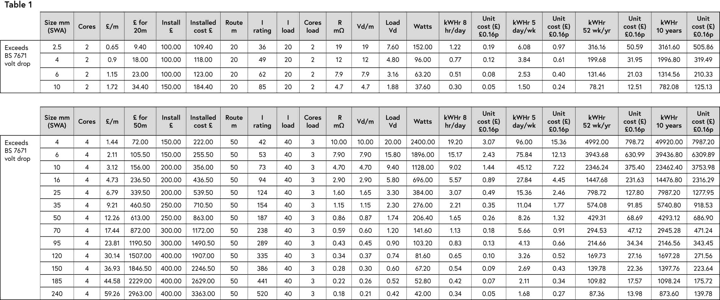
For simplicity, it is assumed that energy consumed is paid for only once a year, at the year-end. In addition, it is widely understood that with inflation, a sum of money spent in the future has less value than an equivalent sum spent now, so there is a ‘present value’ to be calculated for the future energy cost, to allow comparison with current costs (‘future value’). Energy costs are expected to rise over the life of an installation, so an annual energy cost increase should also be included. Finally, there should be a finite installation life for calculation: ten years has been chosen, but in reality, installations may operate for much longer, with resulting increased waste energy costs. (In the longer term it may be a valid proposition to rewire an installation using the same plant, simply to reduce energy costs).
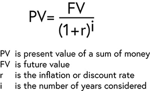
The basic present value of a future sum value can be calculated from the formulae:
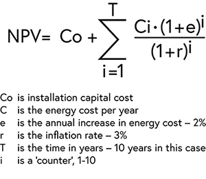
However, to consider the additional annual increase in the cost of energy, at 2%, and the cumulative costs over the ten-year period, the formulae is modified to:
For simple examples, three single-phase and five three-phase loads will be considered further. Looking at Table 2, it can be seen in both the single- and three-phase cases that the most economic installation occurs when the cable installation capital cost and the lifetime energy running cost are effectively equal. In the single-phase installation, the costs are reducing, and it is expected that a 10 sq mm cable would be the optimum. In the three-phase model, the minimum occurs somewhere between a 35 sq mm and a 50 sq mm cable and the final choice would need to be refined by calculation, using specific data for a specific installation.
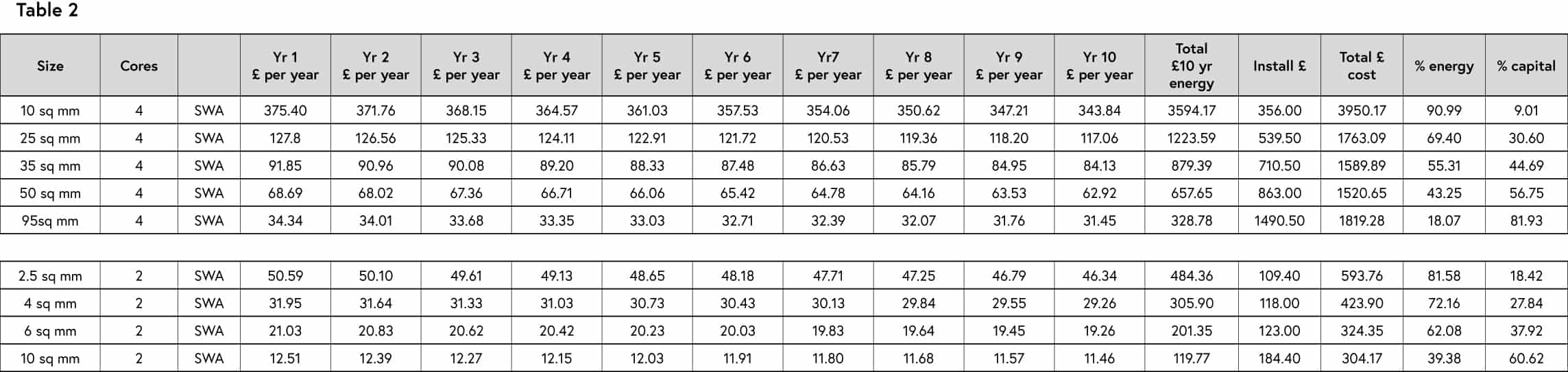
However, any selection of larger conductors will also bring increased cost associated with bigger containment, enclosures, etc. and these will need to be considered in detail for each installation.
Conclusion
As noted previously, this article is only illustrative. More detailed factors applicable to a specific installation would need to be considered in any design. The calculation does, however, show clearly that a smaller cable is not always the most economic choice overall. In the three-phase example, installing a smaller 10 sq mm cable, which could carry the load, could cost the installation owner some £2,400 more in running costs than initially installing a 35 sq mm cable over a ten-year installation life – and that’s just for one cable!
Further investigation into running costs should also be made, as it must be noted that the figures given in the cable rating tables in Appendix 4 of BS 7671 assume a conductor resistance at the full rated current of the cable, whereas a larger conductor carrying less than full rated current will allow the conductor to run cooler, and thus the resistance will be less (the calculation below is very relevant).
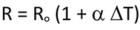
See item 6.1 of Appendix 4 of BS 7671 for further information.
Acknowledgements
[1] Graham Manley, presidential address to the Chartered Institution of Building Services Engineers (CIBSE), 2004.
[2] With assistance from Gary McCafferty, Assistant Manager, Cleveland Cables.
Thanks also to Dr Iain Brock, Shahid Kahn (ECA) and the IET Technical Regulations staff for their helpful comments.